
From the interconnect wall and drive voltage to co-packaging — how efficiency is won a decibel at a time, Interconnect energy in AI clusters: how pJ/bit is measured, why drive voltage matters most, and what each packaging step buys.
Every time a training cluster doubles, the interconnect hanging off it has to move twice as much data. Not so long ago the bottleneck was the compute. Now it is increasingly the movement — not that the maths cannot be done, but that the data cannot be delivered in time. Out of that shift has come a metric harder than bandwidth: picojoules per bit.
This article opens up that bill — where the energy goes, which term is worth attacking, and why the answer is often not in the optical device at all.
1. The interconnect wall
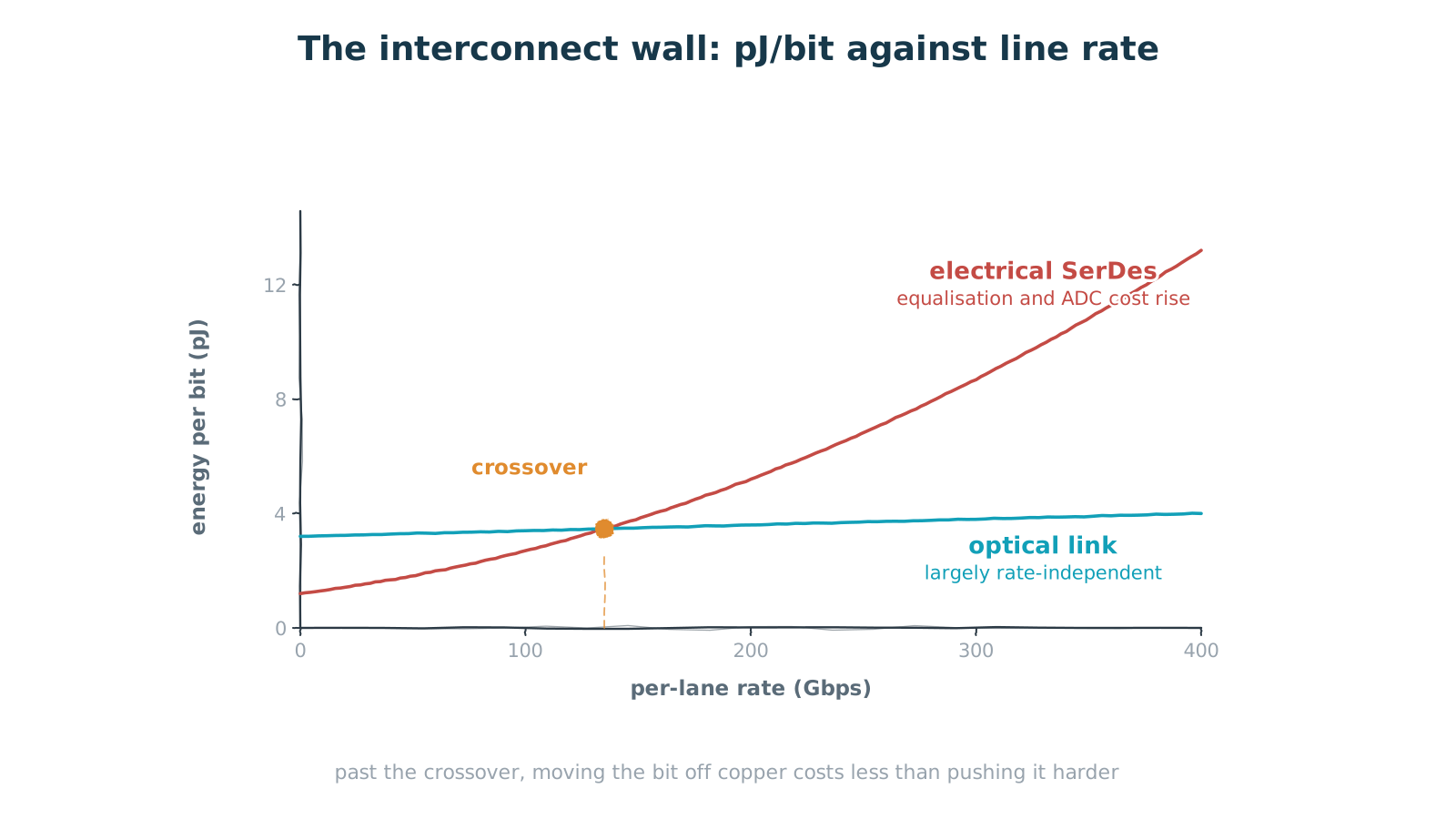
Figure 1 — The interconnect wall: electrical SerDes energy climbs with rate, optical barely moves
past the crossover, pushing harder costs more than changing medium
Plot the problem first. Rate per lane across the axis, energy per bit up the side, and the two lines go in quite different directions.
Electrical SerDes is cheap at low rate — the copper is right next to the die and no conversion is needed. Push the rate up, though, and the costs stack: channel loss grows, so the receiver needs heavier equalisation; when equalisation runs out you reach for an ADC and DSP, and a fast ADC is a hungry block. Energy per bit therefore accelerates with rate.
Optical inverts this. It charges an entry fee — electrical to optical at one end, back again at the other — so at low rates it loses. But that cost is essentially independent of rate: whether you carry 100G or 400G, the wavelength is unchanged and so is the fibre loss.
The two lines must cross, and where they cross is the watershed. Past that point, pushing harder on copper costs more than the fixed overhead of changing medium, and optical starts to win. That is why recent generations have pushed the optical boundary steadily toward the chip — not because light got cheaper, but because electricity got more expensive.
2. Where the energy goes
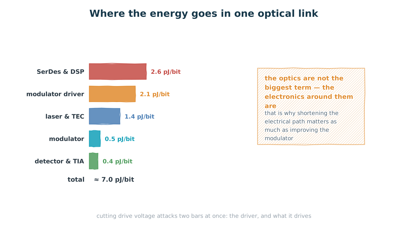
Figure 2 — Where the energy goes in one optical link
the optics are not the biggest term — the electronics around them are
Break down one optical link and the result often surprises: the optics are not the largest term.
Roughly — the SerDes and DSP take the biggest share, the modulator driver comes next, the laser with its temperature control takes another block, and the modulator's capacitive charge-discharge plus the detector and transimpedance amplifier are smallest of all. The modulator term is small precisely because it is mainly a capacitive load and does not dissipate.
Two things follow. First, optimising the optics alone has a low ceiling: halve the modulator's energy and the total moves by only a few percent. Second, the real room is in shortening the electrical path. SerDes and DSP are expensive because the signal has to travel a meaningful distance as electricity, fighting loss and distortion the whole way. Shorten that and both terms fall.
3. Drive voltage: one geometric change, two gains
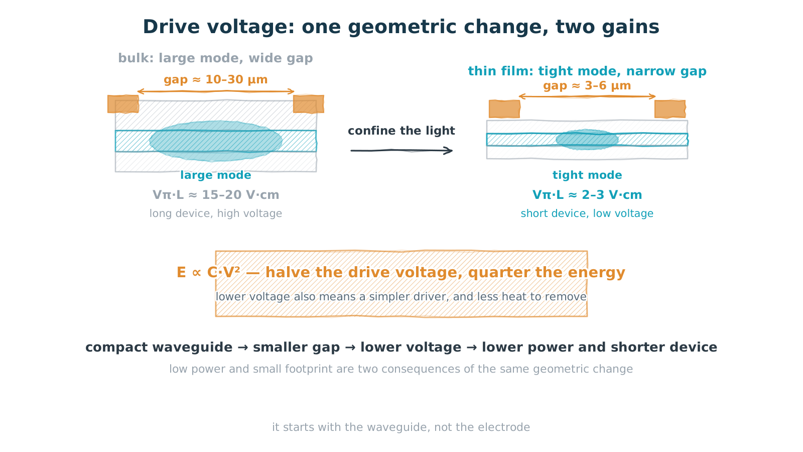
Figure 3 — Drive voltage: one geometric change, two gains
halve the drive voltage and the energy drops by four
So how is the modulator term itself improved? Drive voltage — and the answer to drive voltage lies in waveguide geometry.
A modulator is fundamentally a capacitive load, and the energy spent per switching event goes as CV². Halve the voltage and the energy falls fourfold. Low drive voltage is therefore a squared return, not a linear one.
Drive voltage is set by the electrode gap, and the electrode gap is limited by mode size — the metal cannot come too close or it absorbs the light. In bulk lithium niobate, keeping the guide single-mode means a large mode, so the gap lands in the 10 to 30 micron range, Vπ·L comes out around 15 to 20 V·cm, and you get a long device at high voltage.
Thin-film lithium niobate relaxes that constraint. Confine the light to a sub-micron waveguide and the mode shrinks with it, letting the electrodes sit 3 to 6 microns apart, dropping Vπ·L to roughly 2 to 3 V·cm. One geometric change, two gains: lower drive voltage and shorter device — low power and small footprint are not separate objectives but two faces of the same thing.
There is a third gain that tends to go unmentioned: at lower voltage the driver gets simpler. Drop a gain stage, drop a set of high-voltage parts, and the board-level power and thermal burden fall with it. That is the real value of low drive voltage on the link-level ledger — it takes out two bars of the chart at once.
4. Two networks, two sets of rules
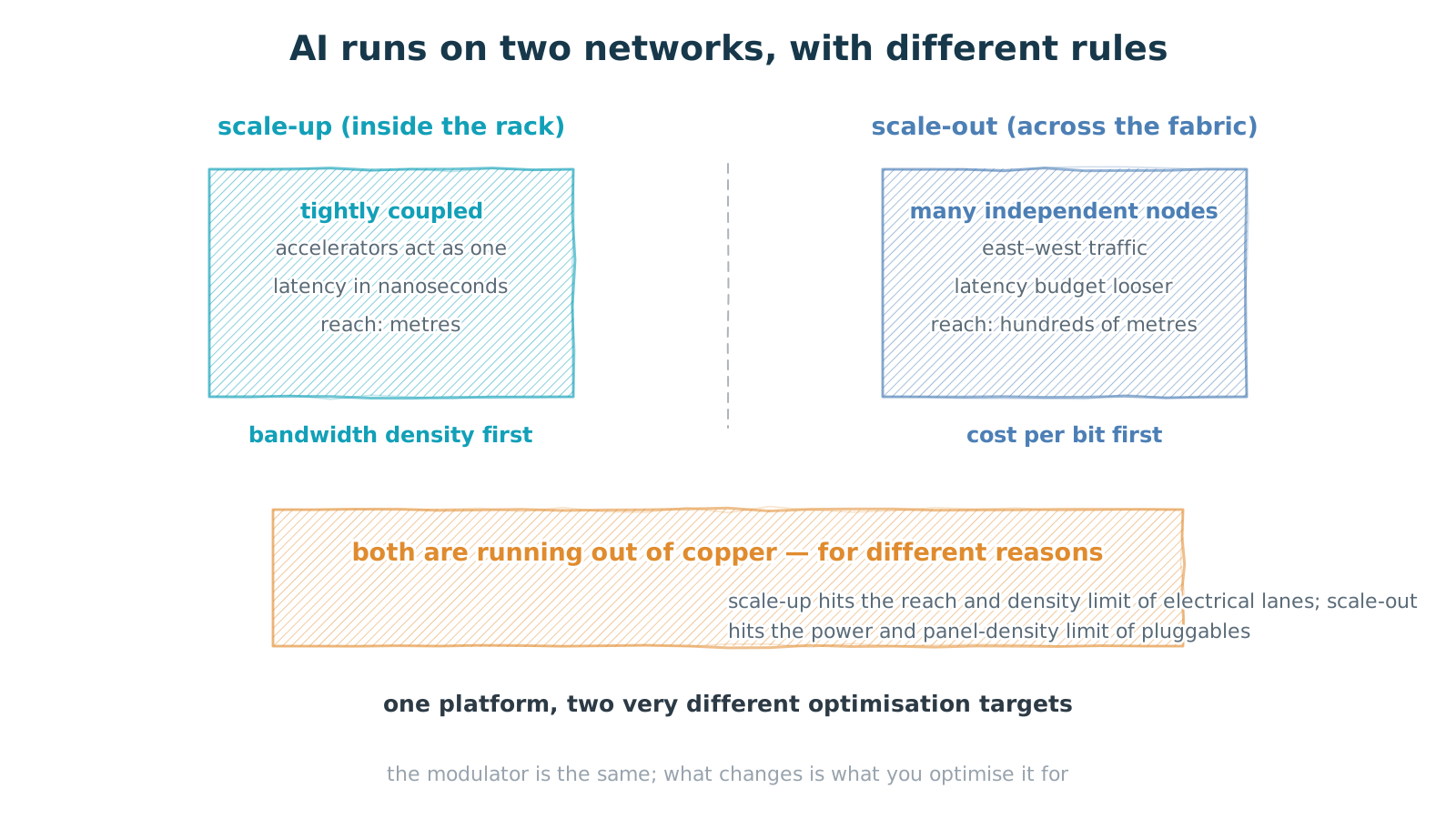
Figure 4 — AI runs two networks with different optimisation targets
scale-up and scale-out run into different limits
A level up, an AI cluster actually runs two networks of quite different character.
Scale-up sits inside the rack, coupling a handful of accelerators tightly enough to behave as one machine. It tolerates nanoseconds, spans a few metres, and wants bandwidth density above all — dense ports, high throughput per unit area. This network runs into the reach and density limits of electrical lanes.
Scale-out spans the fabric, tying together many independent nodes and carrying east–west traffic. The latency budget is far looser and the span runs to hundreds of metres, but the node count is enormous, so cost per bit and faceplate density become the binding constraints. This one runs into the power and density limits of pluggables.
Both are exhausting the headroom in copper, for different reasons. Which is also why one class of optical device serves both — the modulator does not change, the optimisation target does. One side chases bandwidth density, the other cost per bit.
5. Shortening the electrical path
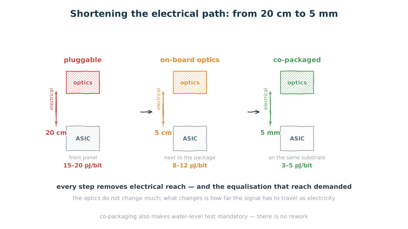
Figure 5 — Shortening the electrical path: from 20 cm to 5 mm
the optics barely change; what changes is how far the signal travels as electricity
If the bulk of the energy sits on the electrical path, the most effective move is to cut that path short. The industry has taken three steps along that line.
First, pluggable: the module sits on the front panel and the signal travels something like 20 cm as electricity before reaching the switch die. That long run is exactly where equalisation and DSP cost comes from, putting the total in the teens of pJ/bit.
Second, on-board optics: move the engine next to the package and the electrical distance compresses to around 5 cm, with energy falling into the high single digits. Third, co-packaged: optics and switch die on a common substrate, leaving 5 mm of electrical interconnect and pushing energy into the low single digits.
Note that the optics barely change across those three steps — it is still the same modulator. What changes is how far the signal has to travel as electricity. That reframing matters: the gain from co-packaging is widely assumed to come from better optics, when in fact it comes from shorter copper.
Co-packaging also imposes a chained requirement: wafer-level test and known-good die. Once the optical part is packaged with the switch there is no rework, and one bad die destroys an expensive assembly, so screening has to happen before dicing. That step was a cost optimisation in the pluggable era; in the co-packaged era it is the price of entry.
6. How efficiency is actually won
Pulling the threads together, a low-power link draws on four directions, with very different weights.
Shortening the electrical interconnect — the largest return, because it removes the two biggest terms outright. Lowering drive voltage — a squared return that takes out the driver and the modulator together. Lowering insertion loss — worth real money on a link budget: a decibel less either buys distance at the same receiver sensitivity, or lets a lower-power laser reach the same place. Raising integration — putting the modulator and a silicon photonics receiver into one module removes interfaces and packaging loss while cutting cost.
That last one has a concrete example. Densely integrating a broadband, compact thin-film lithium niobate modulator with a silicon photonics receiver into a coherent module delivers high output power and high OSNR, and transmission distance improves by roughly 15% over the previous generation. That 15% is not one metric converted — it is several paths adding up, which is also why loss is often worth more than bandwidth at the system level.
On the way to 1.6T the arithmetic only tightens. Lane rates climb, equalisation cost climbs with them, and the energy budget per bit falls rather than rises — so shortening the electrical path and lowering drive voltage carry still more of the load.
Closing
Picojoules per bit looks like a device metric and behaves like a system one. It depends on the modulator, but it depends more on how far the modulator sits from the switch die.
Which means the real efficiency roadmap is not about pushing any single device to its limit. It is about redrawing the boundary between electrical and optical — turning the signal into light as early as possible and making it travel as electricity as little as possible. On that road, device engineering (low drive voltage, low loss, high integration) and packaging (on-board, co-packaged) are two ends of the same thread. Without either one, the other's gains never cash out.
The energy is not in the optics. It is in the stretch of copper between the optics and the die. Cutting that distance is worth more than optimising the modulator one more time.