
Cable loss, single-sideband modulation and true time delay — the engineering logic of microwave photonics, Following RF over fibre: the TFLN IQ modulator, 110 GHz InP detectors, true time delay beamforming and optical heterodyning.
The first wall an RF engineer hits is usually not a component. It is the cable. Push the frequency up and coaxial loss climbs as the square root of frequency — by 60 GHz, a decent run of coax is a few metres long. Optical fibre, by contrast, barely notices frequency at all. Over the same distance the difference in loss runs to two or three orders of magnitude.
That is where RF over fibre starts. What it buys you is loss, weight and immunity; what it costs is two extra electro-optic conversions and a whole set of figures of merit that only an RF engineer thinks to ask about — gain, noise figure and linearity. This article walks through them in that order.
1. Why fibre
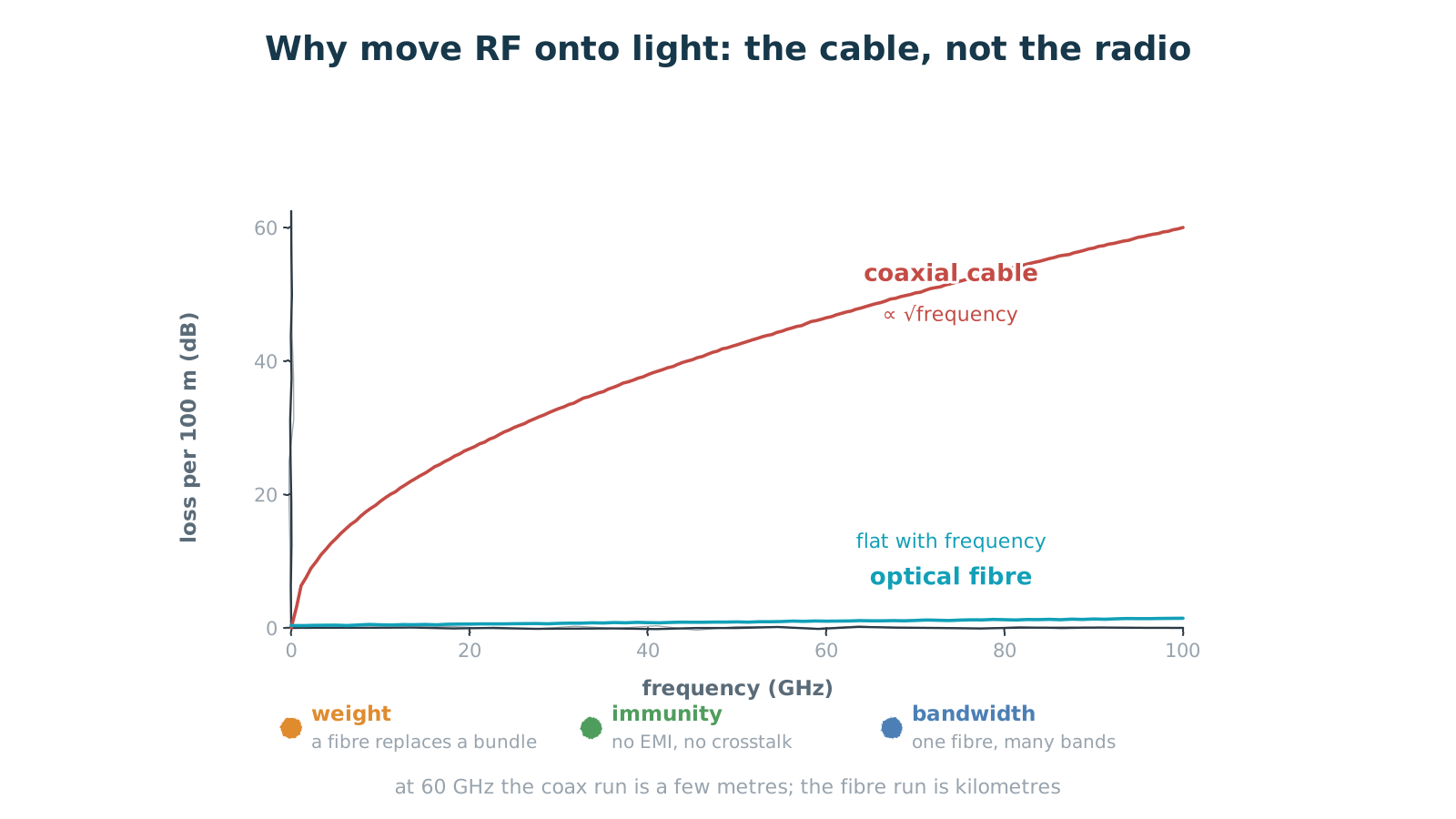
Figure 1 — Coax loss climbs with frequency; fibre barely notices it
a few metres of coax at 60 GHz, or kilometres of fibre
Start with how solid that wall is. Coaxial loss scales roughly with the square root of frequency: quadruple the frequency and the loss doubles. At 60 GHz you are looking at tens of dB per hundred metres, which in practice means a few usable metres. A millimetre-wave system that needs to carry RF from a front end out to a remote unit simply cannot do it over coax.
Fibre is different. At 1550 nm it loses about 0.2 dB per kilometre, and more importantly it is essentially independent of the RF frequency — whether you are carrying 2 GHz or 60 GHz, the optical signal sits at the same optical wavelength and sees the same loss. That frequency independence is the whole point: coax loss rises with frequency and fibre loss does not.
Three things come along for free. Weight — kilometres of fibre weigh far less than the equivalent waveguide or cable run, which matters enormously on airborne and satellite platforms. Immunity — fibre carries no current, radiates nothing and picks up no crosstalk, which removes a great deal of shielding design in electromagnetically hostile environments. And bandwidth — one fibre can carry many RF channels at once by wavelength division, which no cable can do.
2. One device, three jobs
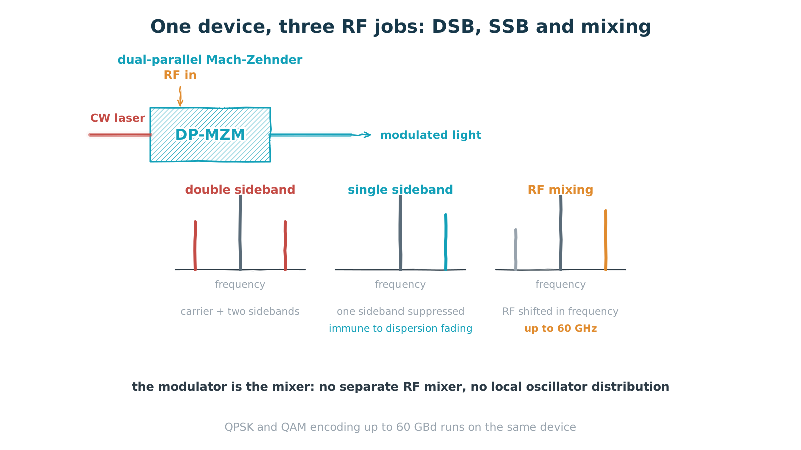
Figure 2 — One device, three jobs: DSB, SSB and frequency mixing
the same part does QPSK and QAM encoding up to 60 GBd
Writing RF onto light is the job of an electro-optic modulator, and RF applications want something different from what telecom wants: linearity. In communications the modulator is driven as a switch and nonlinearity is irrelevant. In an RF link the modulator is a mixer and a linear amplifier, and nonlinearity shows up directly as spurs.
A dual-parallel Mach-Zehnder (DP-MZM) does three things. First, double-sideband modulation: the RF directly modulates the optical intensity, producing a carrier with two sidebands. Simplest possible scheme, but over a long fibre the two sidebands accumulate different phase from dispersion, and their relative phase drifts — which makes the received power fade periodically. That is dispersion fading.
Second, single-sideband modulation: by setting the relative phase and amplitude of the two arms, one sideband is suppressed. It costs drive complexity and buys complete immunity to dispersion fading, which is what you want for long spans. Third, frequency mixing: bias the modulator at the right point and the RF input multiplies with the optical carrier, so the output is the RF shifted in frequency. The modulator is the mixer — no separate RF mixer, no local oscillator distribution network.
Parts like this reach 60 GHz of RF frequency while also supporting QPSK and QAM encoding up to 60 GBd. The same device serves both because the underlying requirements are identical: wide bandwidth, good linearity, low drive voltage.
3. True time delay: the beam stops squinting
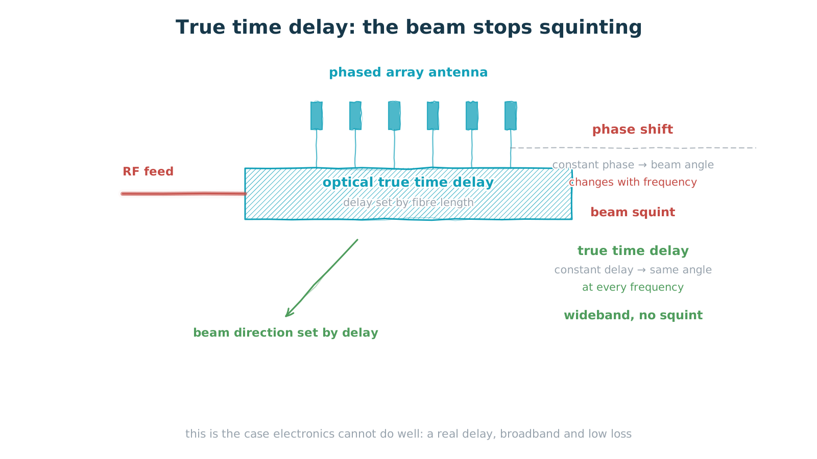
Figure 3 — True time delay: the beam stops squinting
delay comes from fibre length and does not vary with frequency
There is one application electronics handles badly and photonics handles naturally: true time delay.
A phased array steers its beam by controlling the phase at each element. Do that with phase shifters and you are applying a fixed phase offset — but the same phase corresponds to a different amount of time at different frequencies, so the beam points somewhere else as the frequency changes. Different frequency components of a wideband signal point in different directions. That is beam squint, and it is the classic problem of wideband phased arrays.
True time delay instead gives each element a real, frequency-independent delay. Every frequency then sees the same delay, the beam points the same way regardless of frequency, and a wideband signal stays together. And the most natural way to make a true delay is to let light travel different lengths of fibre: the length difference is the delay difference, inherently frequency-independent and almost lossless.
This is why microwave photonics is not merely convenient but irreplaceable in phased-array radar and wideband electronic warfare: not because it is cheaper than the electronic approach, but because the electronic approach cannot hit the specification.
4. Two lasers beat out a millimetre wave
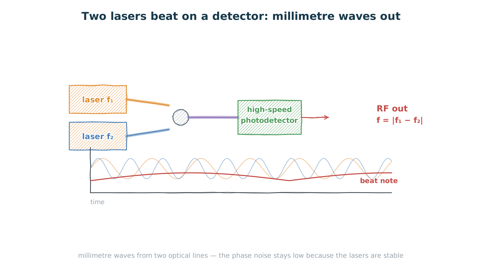
Figure 4 — Two lasers beat on a detector and millimetre waves fall out
the frequency difference is the output; phase noise depends on the lasers
The other thing microwave photonics does exceptionally well is generating millimetre waves with low phase noise.
The method is disarmingly simple. Take two narrow-linewidth lasers at different frequencies, combine them, and send the result to a high-speed photodetector. A detector is a square-law device: its output current is proportional to the square of the optical field, so the difference frequency appears in the output as a beat note. The output RF frequency is the difference between the two optical frequencies.
The appeal is phase noise. An electronic multiplier chain degrades phase noise by 6 dB for every doubling; in the optical approach the phase noise of the millimetre wave is set mainly by the linewidth of the two lasers, so if the lasers are stable the output is clean. Want 60 GHz? Set the frequency difference to 60 GHz — no multi-stage multiplication in between.
Tuning is the other benefit. Shift one laser and the output RF frequency follows, continuously, across a wide range — valuable for fast spectrum analysis and frequency-agile systems.
This places a hard requirement on the detector: bandwidth. Generating a 60 GHz millimetre wave needs a detector with at least 60 GHz of 3 dB bandwidth; volume parts in the 110 GHz class leave comfortable margin. It is also why indium phosphide is the workhorse here, supplying both high-speed, high-power photodetectors and low-noise, high-responsivity InGaAs photodiodes.
5. Bandwidth is only the entry ticket
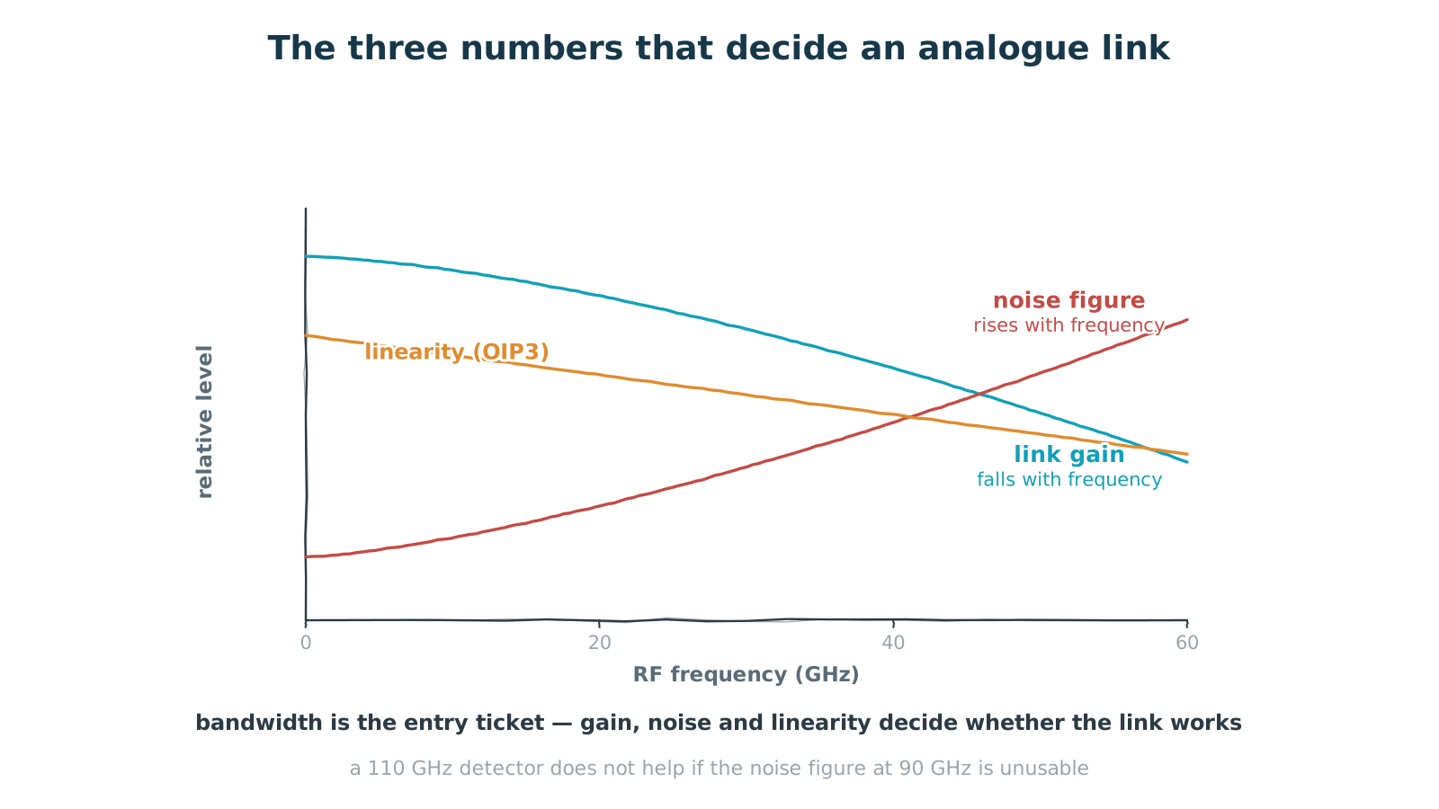
Figure 5 — The three numbers that decide an analogue link
bandwidth gets you in the door; gain, noise and linearity decide
Everything so far has been about what can be done. Whether an analogue optical link is actually usable depends on three other numbers, all of which move with frequency.
Link gain falls with frequency — modulator response, detector response and every impedance match in the chain degrade at the high end. Noise figure rises with frequency: the signal is attenuating while the noise floor is not, so signal-to-noise ratio deteriorates. Linearity, usually quoted as output third-order intercept (OIP3), declines more gently, because at high frequency devices enter their nonlinear region sooner and generate spurs.
Together those three set the dynamic range of the link: the noise figure fixes the floor, linearity fixes the ceiling, and gain decides what sits in between. Quoting 110 GHz of bandwidth on its own tells you very little — if the noise figure at 90 GHz is unusable, a 110 GHz detector does not help.
So RF applications read datasheets differently from communications ones. Bandwidth is not enough; you want gain, noise figure and OIP3 as curves against frequency, plus the optical power and bias conditions they were measured at. Which is the same point the previous article kept making — the conditions matter more than the number.
6. From chip to system
Both ends of this link are products of the same process platform.
On the transmit side, a thin-film lithium niobate electro-optic modulator. The value of the thin film is that the waveguides can be made compact, which shrinks the electrode gap and in turn drops the drive voltage substantially. In an RF link that translates directly into link gain, because the same RF input buys a greater modulation depth. The device also gets shorter, and with a folded optical layout that puts the RF and optical interfaces at opposite ends, the chip stays small and the integrity of the RF feed is far easier to preserve.
On the receive side, an indium phosphide photodetector. It can be supplied as a standalone part or as part of an integrated photonic circuit — both are in volume production, depending on whether a system wants to start from discrete components or integrate on chip. Some 110 GHz of 3 dB bandwidth spans microwave to millimetre wave, and 780 to 2500 nm of wavelength coverage takes in both the O band of datacom and the C band of telecom.
There is a real advantage in sourcing both ends from the same supplier: the modulator's drive voltage, the detector's responsivity and the bandwidth curves of both are designed as a set, so the link budget does not depend on guessing what happens in between. In RF systems, where every decibel has to be accounted for, that is worth having.
Closing
Moving RF onto light is, at bottom, a change of medium: carry electricity down a wire, or carry light down a fibre. What you gain is loss decoupled from frequency, a large drop in weight and immunity to interference. What you pay is the gain, noise and linearity lost in two electro-optic conversions.
At low frequencies the trade does not work — at 2 GHz the coax is fine and there is no reason to add two conversions. As frequency climbs, though, loss on the cable side rises fast and the balance tips quickly. 60 GHz is a clear dividing line, and further into millimetre wave the conclusion only hardens.
Microwave photonics, then, is not trying to replace RF electronics. It takes over where electronics runs out: long-distance transport, true time delay, low phase-noise millimetre-wave generation, and the front end of ultra-wideband analogue-to-digital conversion. Those applications share one thing — each is blocked by a physical limit of cable or of electronic devices, and light happens not to have that limit.
Coax loss climbs with frequency. Fibre loss does not. That single fact decides which path the millimetre waves take.