
The mechanics of quantum frequency conversion — and why background noise, not efficiency, sets the real threshold, Why a telecom-band photon gets moved into the visible, and why background noise — not efficiency — sets the real threshold.
Quantum networking has an awkward constraint built into it. Fibre loss is lowest around 1550 nm, so that is the wavelength a photon should travel at. But detectors work best in the visible — silicon above all, which is cheap, efficient and runs at room temperature. Two requirements, two different wavelengths.
The answer is not to compromise on either. It is to move the photon: let it run the fibre at telecom wavelengths, then change its colour once, at the end of the link. That is quantum frequency conversion. It sounds like a wavelength-conversion problem, but the hard part is not the conversion.
1. The detector sets the wavelength
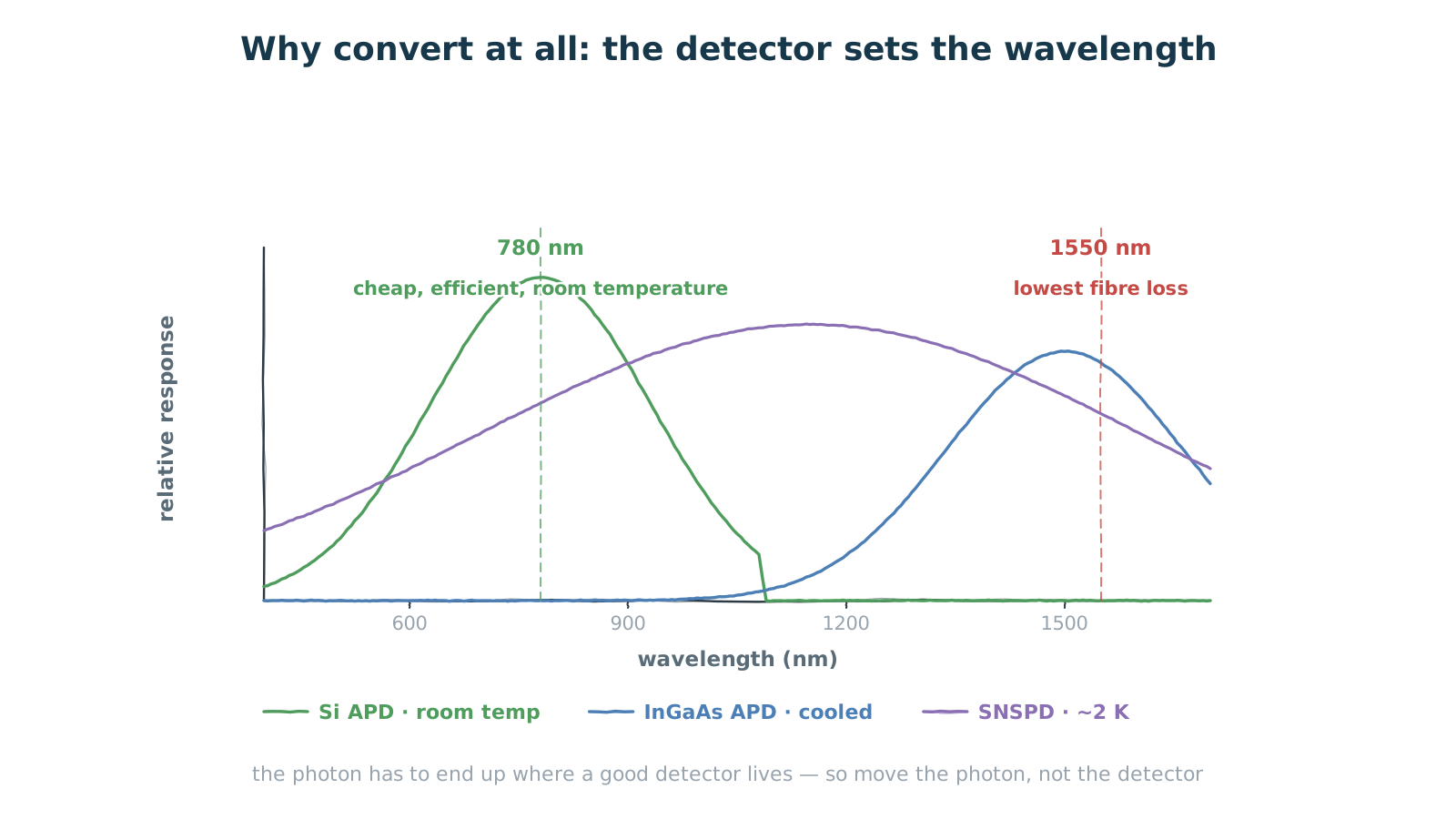
Figure 1 — The detector sets the wavelength: silicon, InGaAs and superconducting options
cheap and room temperature, versus costly, cooled, or at 2 K
Start with why moving it is necessary at all. Three detector families, plotted against wavelength, make the trade obvious.
Silicon detectors (Si APDs) respond best between about 400 and 1000 nm, peaking near 780 nm. They are cheap, efficient and run at room temperature — the least troublesome option by a wide margin. InGaAs APDs cover roughly 900 to 1700 nm and so reach the telecom band, but they need cooling, carry noticeably higher dark counts, and cost considerably more. Superconducting nanowire detectors (SNSPDs) perform best and span the widest range, but they operate at 2 K or below — and the cryogenic system is a burden in its own right.
The choice then becomes arithmetic: either equip every node of the link with an expensive telecom-band detector, or convert once at the end and use cheap silicon throughout. For quantum networks and sensing systems with many detection nodes, the second option scales far better.
The point is not that silicon is a better detector. It is that conversion moves the cost and complexity from the detector to the converter — and the converter is a one-off, reusable, batch-manufactured part, whereas the expensive detector is one you would otherwise need at every node.
2. Upconversion: one signal photon plus a strong pump
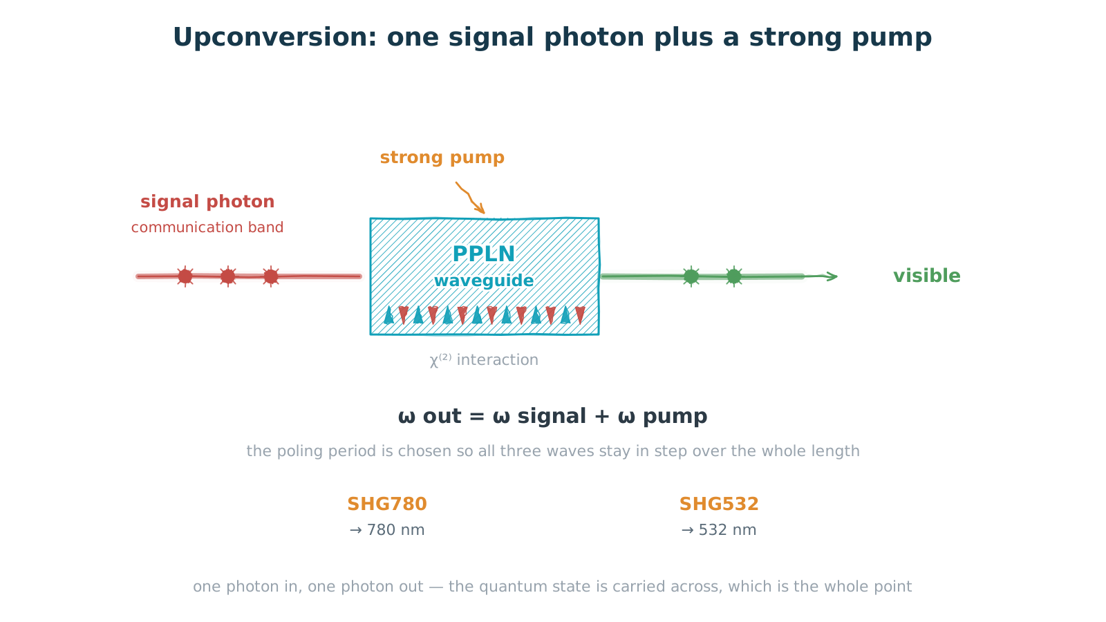
Figure 2 — Upconversion: one signal photon plus a strong pump
the χ⁽²⁾ nonlinearity in a PPLN waveguide, supporting SHG, SFG and DFG
How does a 1550 nm photon become a 780 nm one? Through the second-order nonlinearity in a periodically poled lithium niobate (PPLN) waveguide.
The mechanism is sum-frequency generation: the signal photon interacts with a strong pump field in the waveguide, and the output photon carries the sum of the two frequencies — a shorter wavelength, a bluer colour. Getting useful efficiency out of it requires phase matching, and phase matching is exactly the problem periodic poling solves. Different wavelengths travel at different speeds in the crystal and slip out of step; flip the sign of the nonlinear coefficient every half coherence length and the energy that was about to flow backwards is pushed forward again.
The same physics supports three processes: SHG (second-harmonic generation), SFG (sum-frequency generation) and DFG (difference-frequency generation). They differ in how pump and signal combine — SHG and SFG move a photon up in frequency, DFG moves it down. Which one you use depends on where the photon needs to end up.
The property that matters is that this is one photon in, one photon out. The quantum state — superposition, entanglement, single-photon statistics — is carried across, not measured and re-emitted. That is what gives the technique its value in quantum applications, and why it cannot be replaced by detecting and re-transmitting.
3. The background is the hard part
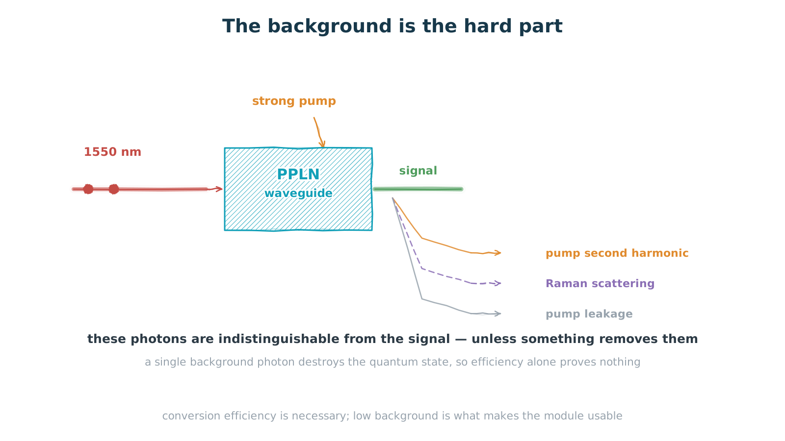
Figure 3 — The background is the hard part
pump second harmonic, Raman scattering and leakage all make signal-coloured photons
All of that is the good news. The trouble is that conversion requires a strong pump, and a strong pump produces a great many photons you did not ask for.
There are at least three sources. First, second-harmonic generation from the pump itself — intense light in a nonlinear material will double its frequency, and that light can land close to the signal wavelength. Second, spontaneous Raman scattering — inelastic scattering of the pump off the crystal lattice, which produces broadband photons spread over a wide wavelength range. Third, pump leakage — no filter rejects the pump completely, and whatever gets through travels straight into the output path.
These photons share the signal's timing, its spatial mode and roughly its wavelength. A detector cannot tell them apart. And in a quantum application, one surplus photon is enough — it contaminates the quantum state, destroys entanglement, and ruins the single-photon statistics.
So conversion efficiency is only a necessary condition. A module with high efficiency and equally high background is useless here: you have moved plenty of signal photons across, but an equal abundance of noise photons came along, and the signal-to-noise ratio has not improved at all. What actually separates one approach from another is low background, and that is usually harder to achieve than high efficiency.
4. Custom wavelength separation
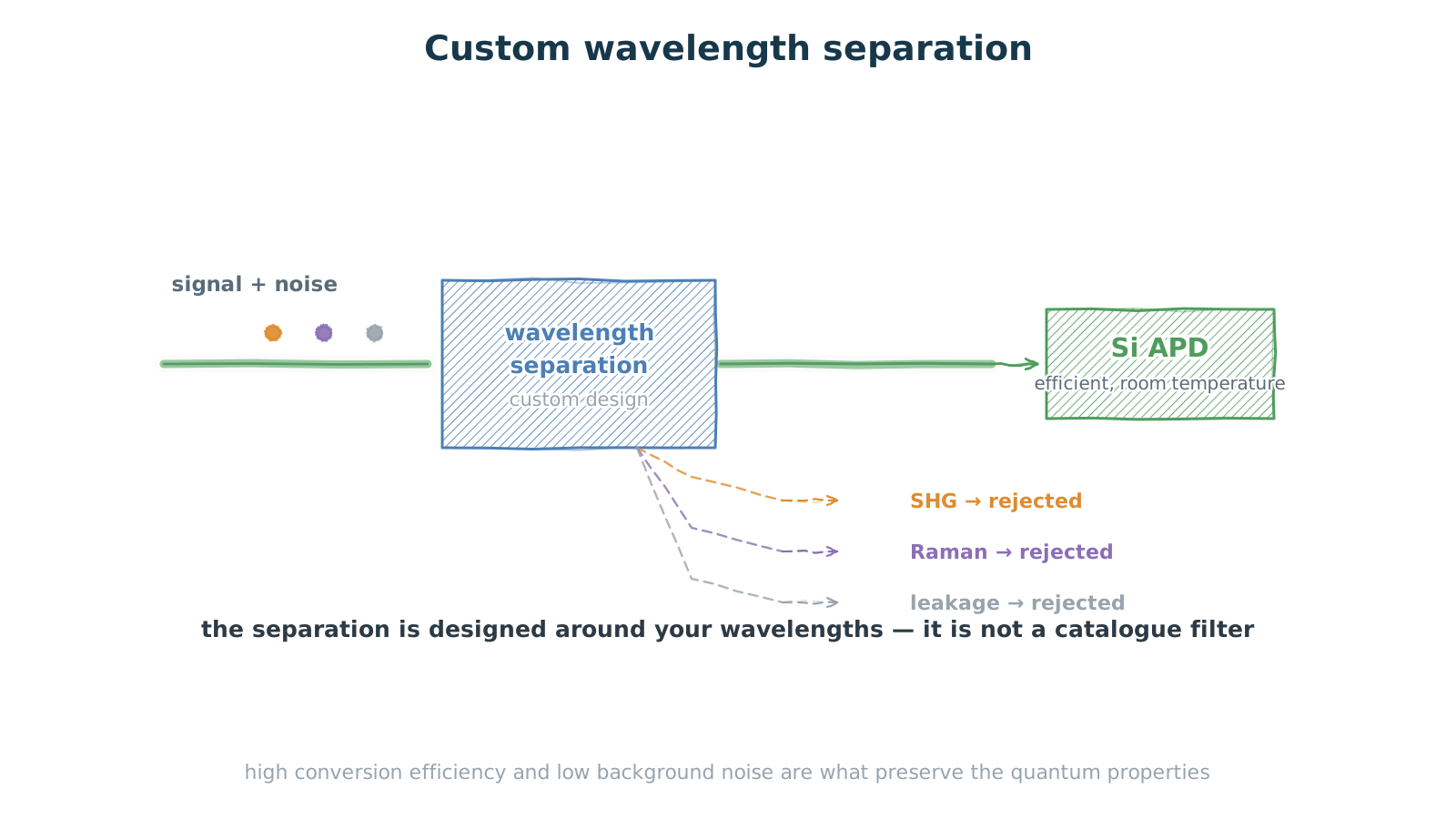
Figure 4 — Custom wavelength separation removes the noise before the detector
designed around your wavelengths, not an off-the-shelf filter
The answer is wavelength separation: dedicated filtering on the output side that removes the by-products before they reach the detector.
Why this cannot be solved with an off-the-shelf bandpass filter is worth stating. The pump's second harmonic, the long tail of Raman scattering and the residual pump light sit very close to the signal in wavelength, and Raman scattering is broadband in the first place. The separation therefore has to be designed around one specific combination of wavelengths — what your pump is, what your signal is, what you are generating — which determines what must be rejected, how much spacing is available, and how many stages are needed.
That is why these modules are custom parts: the separation scheme, like the poling period, is computed for a particular set of wavelengths. Delivering high conversion efficiency and low background together is what preserves the quantum properties of the signal and makes it usable for long-distance quantum communication, networking and sensing.
5. The module, and what to specify
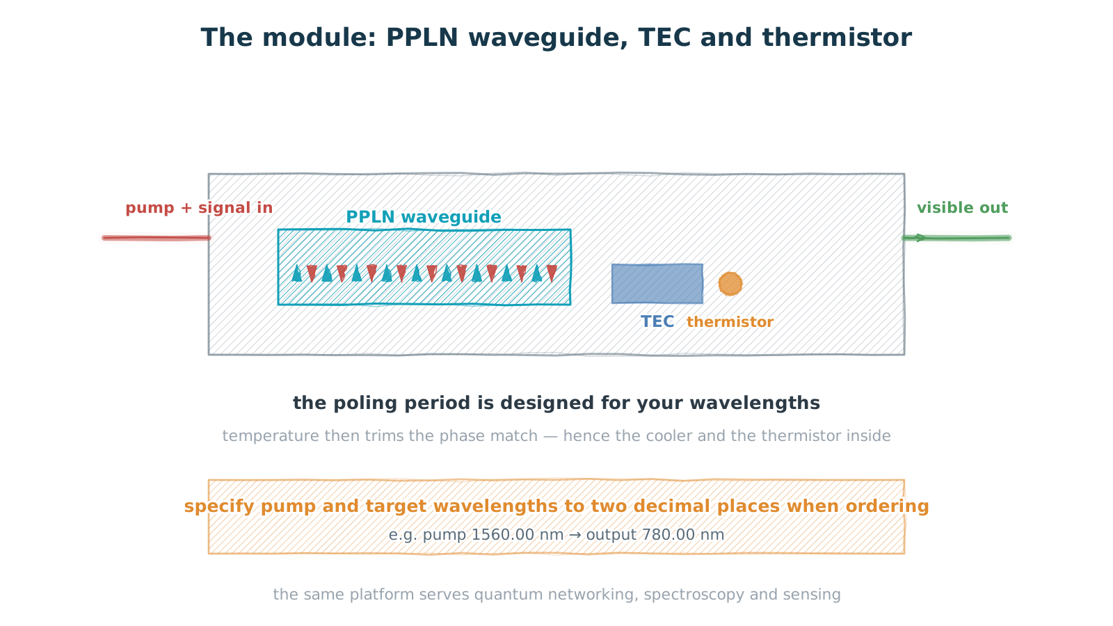
Figure 5 — The module: PPLN waveguide, TEC and thermistor
the period sets the centre wavelength; temperature trims it
In product form, a quantum frequency conversion module contains three things: a PPLN waveguide chip, a thermoelectric cooler (TEC) and a thermistor.
The waveguide chip is the heart of it, and what it buys is interaction strength. Confining the light to a cross-section a few micrometres across holds the intensity high over the whole length, so usable conversion efficiency arrives on a centimetre scale — orders of magnitude away from what a bulk crystal does.
The TEC and thermistor are not accessories. Phase matching is temperature-sensitive, and once the poling period is fabricated it cannot be changed, so temperature is the only trim available. Temperature control is also what holds the wavelength steady over long runs.
Which makes the poling period the parameter that defines a custom part. Given a pump wavelength and a target wavelength, the required period follows. Insisting on pump and target wavelengths to two decimal places when ordering is not bureaucracy — those two numbers determine the period, and the period determines whether the module works at your wavelengths at all.
Worth noting how the modules are named: by output wavelength. SHG780 delivers 780 nm, SHG532 delivers 532 nm. Both land in the region where silicon detectors respond well.
6. What to hand over when ordering
Pulling the above together, the list of things to specify is short, but none of the entries can be vague.
Modules are named for their output — SHG780, SHG532 — so start there. Pump wavelength and target output wavelength, both to two decimal places; if you are using SFG or DFG, say which process. The input signal wavelength, usually somewhere in the telecom band. The by-products to reject — where the pump's second harmonic lands, how far the Raman tail extends. Your operating temperature and stability requirement. And the detector type, since that decides which output wavelength to optimise for.
One more question worth asking: is there measured data on low background, or only on conversion efficiency? The two matter very differently in quantum applications, and efficiency is the number that tends to sit at the front of a datasheet.
Closing
Quantum frequency conversion is a good illustration of a broader point: quantum applications judge devices by entirely different criteria than the data centre does. A communications link asks about power per bit. A quantum link asks how clean the result is — whether the photon can be moved without anything else being mixed in along the way.
A converter that moves photons quickly and precisely but sheds noise the whole way is less useful than a slower, clean one. Which is why, in this corner of the field, low background deserves top billing more than high conversion efficiency does.
Communications asks how much you moved. Quantum asks how much you contaminated. Efficiency decides the first; background decides the second.