
The first two articles were about one thing: how light moves bits from A to B. That is the main thread of the last decade in photonics — bandwidth, power, cost per bit, every metric orbiting that one story. But the same crystal has a second career entirely.
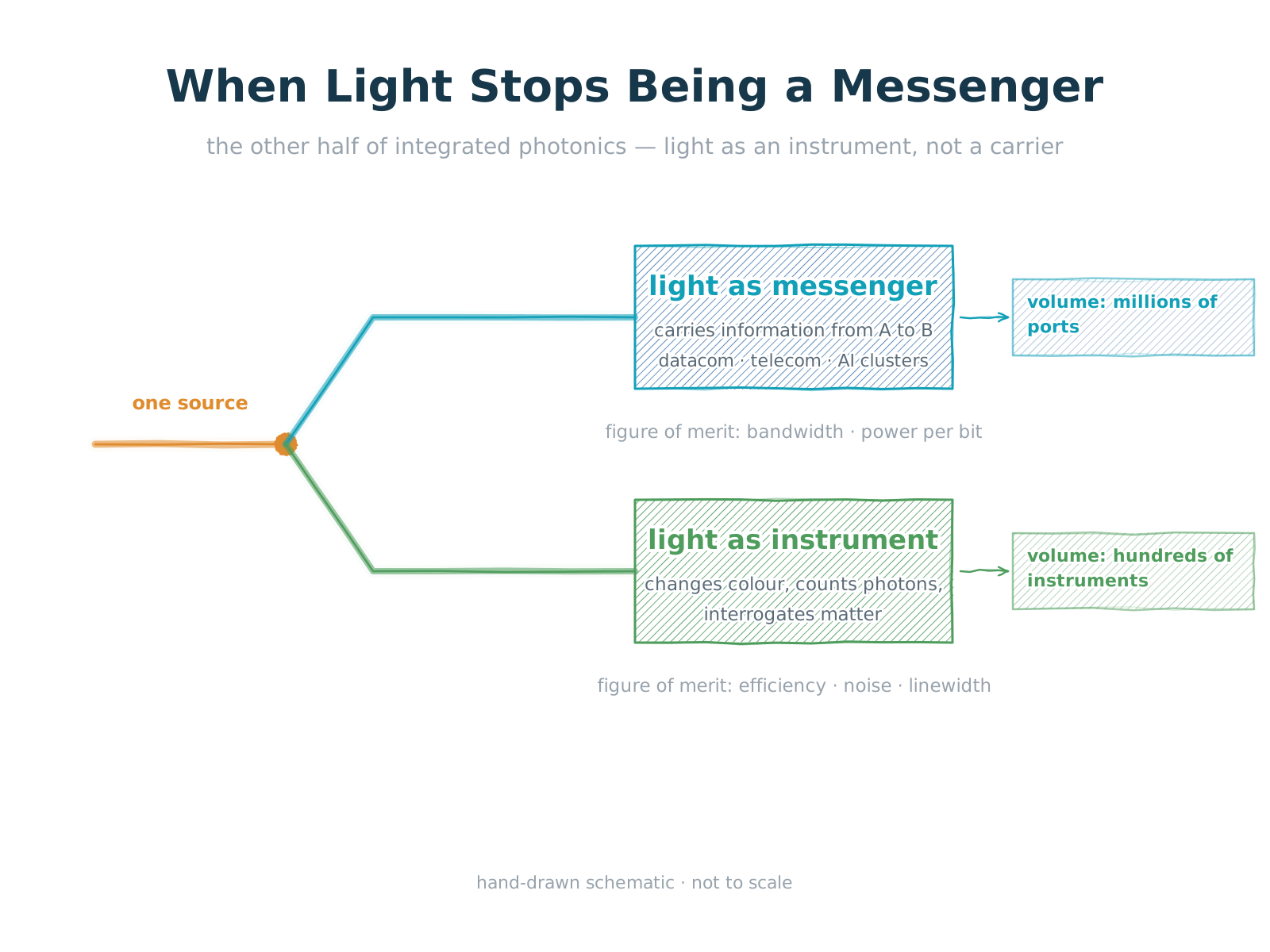
Instead of carrying information, the photon itself becomes the object of manipulation: change its colour, count how many there are, use it to ask matter a question. This half ships in hundreds of instruments rather than millions of ports, yet in some dimensions it demands more of the device, not less. This article is about that half.
1. Two jobs for one photon
The distinction is this. As a carrier, the photon is a container. We care how fast it arrives and how much energy the trip costs; what wavelength it happens to be, or how clean its phase is, matters only insofar as the receiver can still read it.
As an instrument, the photon is what is being operated on. Wavelength is an output to be controlled precisely. Coherence is a resource to be preserved. The number of stray photons is a figure to be pushed below one.
Two different objective functions, and therefore two different definitions of a good device: bandwidth and joules per bit on one side, conversion efficiency, background and linewidth on the other. Same crystal; the two rulers do not give the same answer.
2. Changing the colour: the waveguide buys orders of magnitude
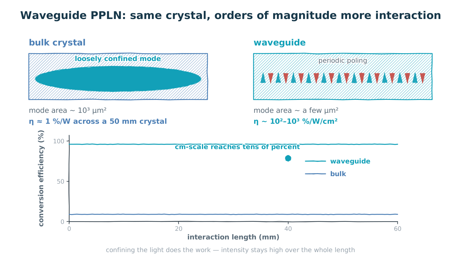
Figure 1 — Bulk crystal vs. waveguide PPLN: same crystal, orders of magnitude more interaction
confinement holds the intensity high over the whole length
Turning 1550 nm into 780 nm relies on the second-order nonlinearity, and the obstacle is phase matching. Light of different wavelengths travels at different speeds in the crystal, so the fundamental and the second harmonic slip out of step, energy sloshes back and forth, and net conversion efficiency goes nowhere.
Quasi-phase-matching sidesteps this. If the mismatch accumulates, flip the sign of the nonlinear coefficient every half coherence length so the energy that was about to flow backwards gets pushed forward again. Physically that means periodic poling: a high-voltage field produces alternating ferroelectric domains in lithium niobate — PPLN.
What changed the economics was making it a waveguide. In a bulk crystal the mode area is on the order of 10³ µm² and the intensity cannot be raised; in a waveguide the mode collapses to a few µm², so over the same length the intensity is one to two orders of magnitude higher and the interaction strength rises by two to three. A bulk crystal needs tens of millimetres to reach a few percent normalised efficiency; a waveguide reaches double-digit percent on a centimetre scale. The knock-on benefit is that pump power requirements fall — a watt-level pump gives usable output, and the module can be sealed with its own temperature control.
3. One crystal, many colours
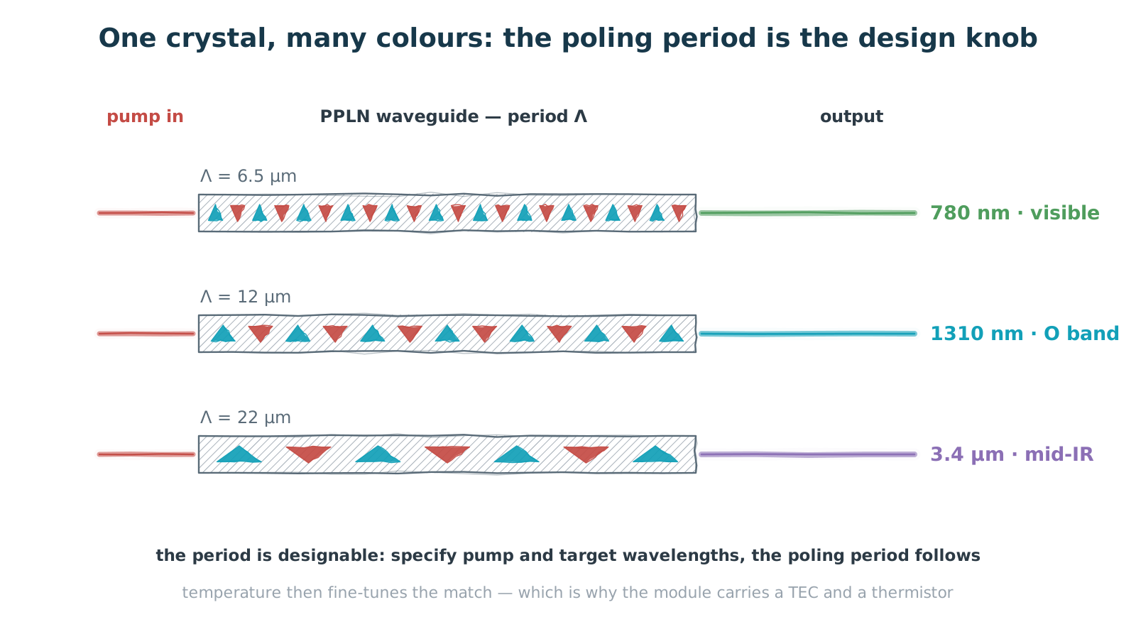
Figure 2 — The poling period is a design degree of freedom: visible, near-IR and mid-IR from one crystal
the period sets the centre wavelength; temperature trims it — hence the TEC and thermistor in every module
QPM has a second virtue: the period is designable. Given a pump wavelength and a target wavelength, the required poling period follows. One process line, different periods, and out come visible, near-infrared and mid-infrared.
The visible band — 780 nm, say — sits right where silicon detectors are most sensitive. 1310 nm is the home turf of data communications. Push further out and 3–5 µm is the mid-infrared fingerprint region, where many gases absorb strongly.
The period sets the centre wavelength; temperature trims it, which is why every module carries a TEC and a thermistor. Specifying pump and target wavelengths to two decimal places when ordering is not bureaucracy — those two numbers are what determine the poling period. And the period is a design degree of freedom where temperature is only a correction. Once that relationship is clear, it is easy to see why this product family is inherently many-variety, small-batch.
4. Moving a single photon
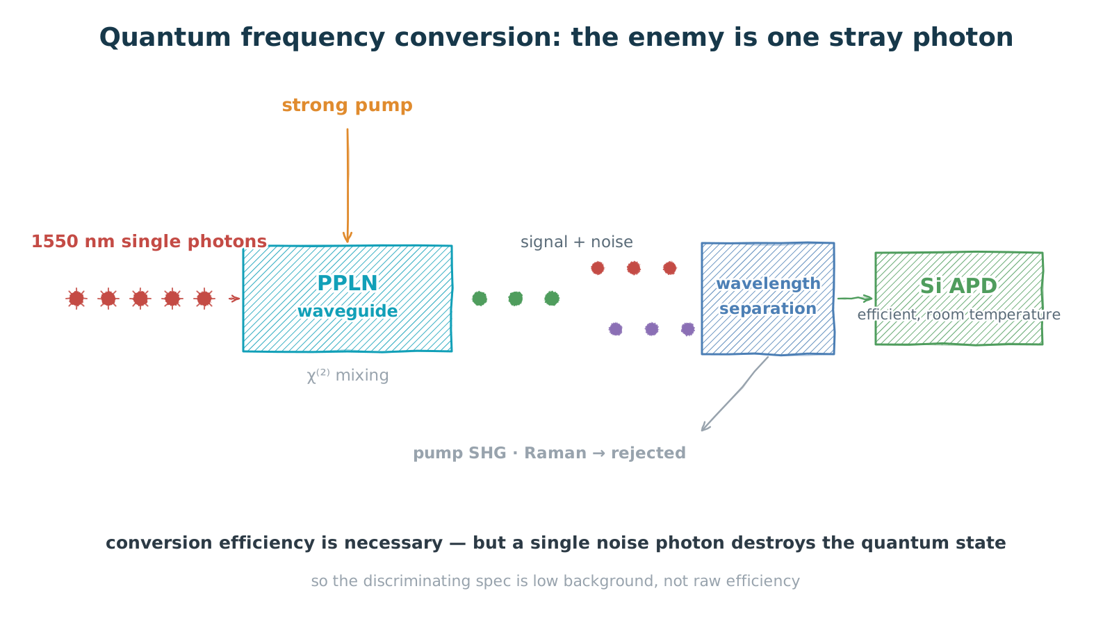
Figure 3 — Quantum frequency conversion: the hard part is not efficiency, it is one stray photon
efficiency is necessary; the real threshold is low background
Quantum frequency conversion is perhaps the most counter-intuitive item in the portfolio. If fibre loss is lowest at 1550 nm, why move the photon at all?
The answer sits at the detector. Silicon single-photon detectors are efficient, cheap and operate at room temperature — but they perform best in the visible, particularly around 780 nm. At 1550 nm you are pushed back onto expensive, deeply cooled detectors. So convert once at the end of the link, move the telecom-band photon into the visible, and detect it with cheap silicon.
The difficulty is that this is conversion at the single-photon level. Second-harmonic generation from the strong pump leaves background photons; so does spontaneous Raman scattering. Any surplus photon contaminates the quantum state, destroying entanglement and single-photon statistics. Hence the dedicated wavelength-separation design that filters these by-products out before they reach the detector.
In other words: conversion efficiency is necessary, but what separates one approach from another is low background. Those two are usually harder to deliver together than raw power efficiency.
5. Using light to measure
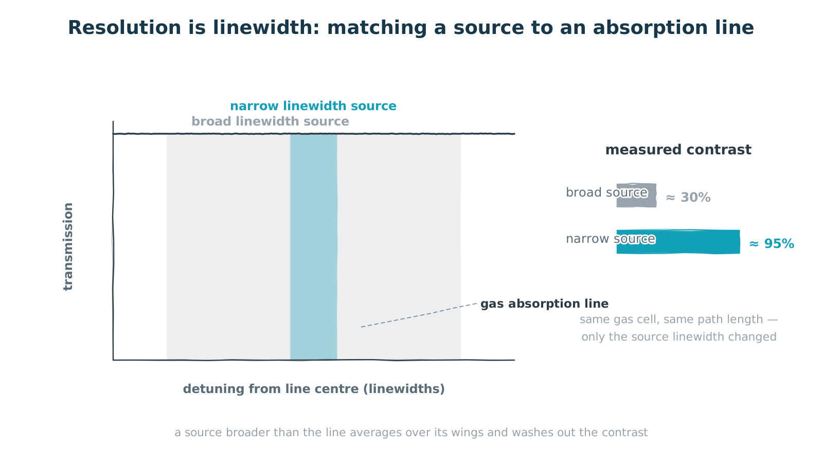
Figure 4 — Resolution is linewidth: matching a source to a gas absorption line
same gas cell, same path — only the linewidth changed
Spectroscopy wants something entirely different from a source than communications does. Communications cares about modulation rate; spectroscopy cares about linewidth, because resolution is linewidth.
Take a gas absorption measurement. The absorption line has a finite width. If the source is much broader than the line, its power is spread across the wings and only a small slice in the middle is actually absorbed, so the measured contrast is diluted. If the source is narrower than the line, nearly all the light lands where absorption is strongest, and the contrast appears.
Same gas cell, same path length, only a narrower source: measured contrast can jump from roughly thirty percent to above ninety. That is why narrow-linewidth sources are a hard requirement in gas spectroscopy and environmental monitoring rather than a nice-to-have. The same logic appears in ultrafast sources: fluorescence spectroscopy wants picosecond or femtosecond pulses at a specific wavelength, and pulse width and wavelength stability are the metrics that matter.
6. The analogue world
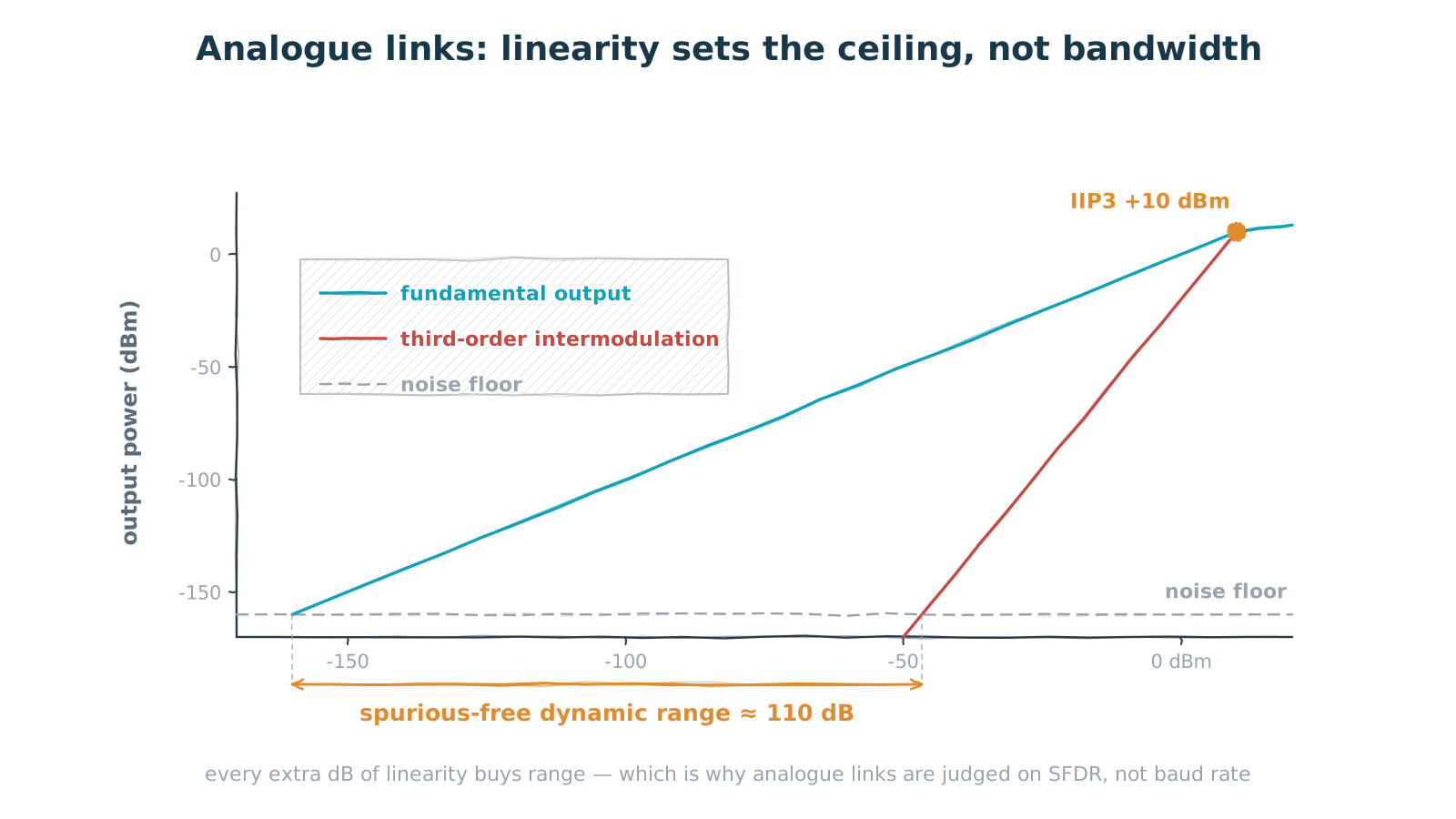
Figure 5 — The classic analogue metric: SFDR, bounded by the noise floor, the fundamental and third-order intermodulation
the fundamental rises 1 dB per dB, third-order intermod 3 dB per dB
The last few sections were digital, or about counting photons. A large block of applications is neither: microwave photonics. Modulate a radio-frequency signal onto light, transport and process it over fibre, then demodulate back to RF.
The benefits are direct: fibre loss is very low and essentially independent of frequency, bandwidth is enormous, and the link is immune to electromagnetic interference. A set of functions that are hard to do in pure RF become feasible — fast spectrum analysis, low-phase-noise microwave and millimetre-wave generation, high-frequency conversion, long true-time delay, and the front end of ultra-fast analogue-to-digital conversion.
But the figure of merit is completely different from a digital link. Digital counts bit errors; analogue cares about linearity, because any nonlinearity produces intermodulation distortion, and once an intermodulation product lands inside the signal band it cannot be filtered out.
The classic metric for an analogue link is spurious-free dynamic range (SFDR), and three things bound it: the noise floor, the fundamental output, and the third-order intermodulation product. The fundamental rises one decibel per decibel of input; third-order intermod rises three. They meet at the input third-order intercept point, IIP3, and the dynamic range is the span from the noise floor up to where intermod touches it. The conclusion is slightly counter-intuitive: the ceiling on an analogue link is usually linearity, not bandwidth. Every extra decibel of linearity buys another slice of usable range.
Closing: two rulers
Read these sections together and a pattern appears. These applications ship in volumes orders of magnitude below the data centre, yet in some dimensions they demand more of the device — higher efficiency, lower background, narrower linewidth, better linearity.
They share the same underlying physics: the second-order nonlinearity of lithium niobate, periodic poling, waveguide confinement, thermal stability. They also share one engineering reality: these metrics resist being maximised simultaneously, so selecting a part means knowing which one you are willing to concede.
Digital links ask "how fast, how cheap". Analogue and quantum applications ask "how clean". Same crystal, two different rulers.